BERT4Rec
Created: 2022-06-20 17:23
#paper
Main idea
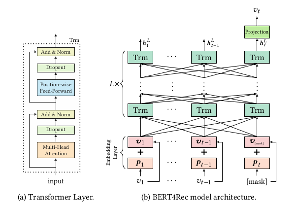
BERT4Rec is a lot like regular BERT for NLP. In this case the Transformer network is trained to predict masked items (Cloze Task) from a user’s history. Then, the self-attention is what allows this architecture to model long-range dependencies between elements of the input sequence.
To use the Cloze task in a sequential recommender the authors added the special masked token to the end of each input sequence to represent the item that has to be recommended and then made recommendations base on its final hidden vector.
In deep
Notation: $U={u_1,u_2,...,u_{|U|}}$ is a set of users, $V={v_1,v_2,...,v_{|V|}}$ a set of items and $S_u=[v_1^{(u)},...,v_t^{(u)},...,v_{n_u}^{(u)}]$ is the interaction sequence in chronological order for user $u \in U$, where $v_t^{(u)} \in V$ is the item that u has interacted with at time step t and $n_u$ is the length of interaction sequence for user u. The goal is then to predict the item the user u will interact with at time step $n_u+1$ -> $p(v_{n_{u+1}}^{(u)}=v|S_u)$.
Transformer Layer
Given an input sequence of length t we iteratively compute hidden representations $h_i^l$ at each layer l for each position i simultaneously by applying the Transformer layer. The representations are then stacked together into a matrix $H^l \in R^{t \times d}$ since we compute the attention function on all the positions simultaneously.
The Transformer layer is divided in two sub-layers:
- Multi-Head Self-Attention: it is used because it is beneficial to jointly attend to information from different representation subspaces at different positions. It works by linearly projecting $H^l$ into h subspaces, using several learnable projections, and then apply h attention functions in parallel to produce the output representations which are concatenated and again projected -> $MH(H^l)=[head_i;head_2;...;head_h]W^O$, where $head_i=Attention(H^lW_i^Q,H^lW_i^K,H^lW_i^V)$ and $W_i^Q \in R^{d \times d/h}, W_i^K \in R^{d \times d/h}, W_i^V \in R^{d \times d/h}$ and $W_i^O \in R^{d \times d}$ are learnable parameters. The Attention Function used is a Scaled Dot-Product Attention: $Attention(Q,K,V)=softmax(\dfrac{QK^T}{\sqrt{d/h}})V$ and Q,K and V are projected from the same matrix $H^l$ with different learned projection matrices. The temperature $\sqrt{d/h}$ produces a softer attention distribution for avoiding extremely small gradients;
- Position-wise Feed-Forward Network: it is important to introduce nonlinearity and interactions between different dimensions in the model. It consists of two affine transformations with a Gaussian Error Linear Unit (GELU) activation: $PFFN(H^l)=[FFN(h_1^l)^T;...;FFN(h_t^l)^T]^T$ with $FFN(x)=GELU(xW^{(1)}+b^{(1)})W^{(2)}+b^{(2)}$ and $GELU(x)=x \Phi(x)$ where $\Phi(x)$ is the cumulative distribution function of the standard gaussian distribution, $W^{(1)} \in R^{d \times 4d}, W^{(2)} \in R^{4d \times d}, b^{(1)} \in R^{4d}$ and $b^{(2)} \in R^d$ are learnable parameters and shared across all positions.
The self-attention layers are then stacked, residual connection is used around the two sub-layers and layer normalization and droupout are also used. This means that the output of each sub-layer is $LN(x + Dropout(sublayer(x)))$, where sublayer(·) is the function implemented by the sub-layer itself, LN is a layer normalization function. The authors use LN to normalize the inputs over all the hidden units in the same layer for stabilizing and accelerating the network training.
Embedding Layer
In order to make use of the sequential information od the input, we inject the Positional Embeddings into the input item embeddings at the bottom of the Transformer layer stacks. The input representation $h_i^0$ of the item $v_i$ is given by $h_i^0=v_i+p_i$ where $v_i \in E$ is the d-dimensional embedding for item $v_i$ and $p_i \in P$ is the d-dimensional positional embedding for position index i. The authors used learnable positional embeddings instead of a fixed sinusoid embedding. The positional embedding matrix $P \in R^{N \times d}$ allows th emodel to identify which portion of the input is dealing with. However, this kind of positional embedding imposes a restriction on the maximum sentence length that the model can handle.
Output Layer
At the end of the previous layers we get the final output $H^L$ for all item of the input sequence. If the masked item is $v_t$, then the want to predict it based on $h_t^ L$ by applying a two-layer feed-forward network with GELU activation in between that produces an output distribution over trget items.
Cloze task
It is used to solve the problem of prediction with bidirectional models. In each training step, $\rho$ proportion of all items in the input sequence are randomly masked and then the model predict the originals ids of the masked items based only on its left and right context. The final hidden vectors corresponding to the mask label are fed into an output softmax over the item set. The loss for each masked input $S_u'$ is defined as the negative log-likelihood of the masked targets: $L=\dfrac{1}{|S_u^m|}\sum_{v_m \in S_u^m} -\log P(v_m=v_m*|S_u')$, where $S_u'$ is the masked version of user behavior history $S_u$, $S_u^m$ is the set of random masked items in it, $v_m*$ is the true item for the masked item $v_m$ and P() is the probability defined in the output.
An additional advantage of the Cloze task i that it can generate more samples to train the model (if we have n samples and we randomly mak k items, we can obtain up to $\binom{n}{k}$).
Results
BERT4Rec outperforms all the SOTA models in every dataset that the authors tried.
The cause of this can be found in the use of bidirectional representations. Cloze task also helps to improve performances.
The number of masked items depends on the length of the sequences, i.e. with longer sequences we need a bigger $\rho$, since a big $\rho$ in longer sequences means much more items that need to be predicted.
Furthermore, user's behavior is affected by more recent items on short sequence datasets and less recent items for long sequence datasets.
Conclusion
BERT4Rec beats every other SOTA model, but it does not consider item features (just item IDs) and it does not explicitly model users.